Which Is Better For Lower Back Training Clean Jerk Vs Power Clean

Effect of batch size on training dynamics

This is a longer blogpost where I discuss results of experiments I ran myself.

In this experiment, I investigate the effect of batch size on training dynamics. The metric we volition focus on is the generalization gap which is divers as the difference between the train-time value and test-fourth dimension value of a metric you care nigh. We volition investigate batch size in the context of image classification. Specifically, we volition utilize the MNIST dataset. In our case, the generalization gap is merely the difference between the nomenclature accuracy at test time and train time. These experiments were meant to provide some basic intuition on the furnishings of batch size. It is well known in the motorcar learning community the difficulty of making full general statements well-nigh the effects of hyperparameters as behavior often varies from dataset to dataset and model to model. Therefore, the conclusions we make tin can but serve as signposts rather than full general statements about batch size.

Some relevant papers on the topic of the batch size and generalization gaps include (some of my experiments reproduce the results in these papers):

• Don't disuse the learning rate increase the batch size
• Train longer, generalize better: closing the generalization gap in big batch training of neural networks

Batch size is one of the near important hyperparameters to melody in modern deep learning systems. Practitioners oft want to employ a larger batch size to train their model as it allows computational speedups from the parallelism of GPUs. However, it is well known that as well large of a batch size will pb to poor generalization (although currently information technology's not known why this is and then). For convex functions that we are trying to optimize, there is an inherent tug-of-state of war betwixt the benefits of smaller and bigger batch sizes. On the ane extreme, using a batch equal to the entire dataset guarantees convergence to the global optima of the objective role. However, this is at the toll of slower, empirical convergence to that optima. On the other hand, using smaller batch sizes accept been empirically shown to take faster convergence to "good" solutions. This is intuitively explained by the fact that smaller batch sizes allow the model to "start learning before having to meet all the data." The downside of using a smaller batch size is that the model is non guaranteed to converge to the global optima. It will bounce effectually the global optima, staying outside some ϵ-ball of the optima where ϵ depends on the ratio of the batch size to the dataset size. Therefore, under no computational constraints, information technology is ofttimes advised that 1 starts at a pocket-size batch size, reaping the benefits of faster training dynamics, and steadily grows the batch size through preparation, likewise reaping the benefits of guaranteed convergence.

The picture is much more nuanced in non-convex optimization, which nowadays in deep learning refers to any neural network model. It has been empirically observed that smaller batch sizes non only has faster training dynamics but also generalization to the examination dataset versus larger batch sizes. But this argument has its limits; we know a batch size of 1 unremarkably works quite poorly. It is generally accepted that there is some "sweetness spot" for batch size betwixt 1 and the entire training dataset that will provide the best generalization. This "sweet spot" usually depends on the dataset and the model at question. The reason for better generalization is vaguely attributed to the existence to "racket" in small-scale batch size training. Considering neural network systems are extremely prone overfitting, the thought is that seeing many small batch size, each batch being a "noisy" representation of the entire dataset, will cause a sort of "tug-and-pull" dynamic. This "tug-and-pull" dynamic prevents the neural network from overfitting on the training set and hence performing badly on the test set.

In some ways, applying the analyse tools of mathematics to neural networks is analogous to trying to apply physics to the study of biological systems. Biological systems and neural networks, are much too complex to describe at the individual particle or neuron level. Often, the all-time we can exercise is to apply our tools of distribution statistics to acquire about systems with many interacting entity. However, this almost always yields a coarse and incomplete agreement of the system at hand. This study is no exception.

Trouble statement

The precise problem that will be investigated is one of classification. Given an image X , the goal is to predict the label of the epitome y. In the case of the MNIST dataset, X are black-and-white images of the digits 0 to 9 and y are the corresponding digit labels "0" to "9". Our model of option is a neural network. Specifically, nosotros volition use a multi-layer perceptron (MLP) or informally "your average, vanilla neural network."

Unless otherwise stated, the default model was used:

• 2 fully connected (FC) hidden layers, 1024 units each
• ReLU nonlinearities
• loss: negative log likelihood
• optimizer: SGD
• learning rate: 0.01
• epochs: 30

Ultimately the question nosotros want to respond is "what batch size should I utilise when training a neural network?"

Outcome of batch size

For sanity sake, the first thing nosotros ought to practise to ostend the problem we are trying to investigate exists by showing the dependence between generalization gap and batch size. I've been referring to the metric we care about equally the "generalization gap." This is typically the measure of generalization authors utilize in papers merely for simplicity in our study nosotros only care nigh the test accuracy existence equally high as possible. As we will come across, both the grooming and testing accuracy volition depend on batch size then it's more meaningful to talk about examination accuracy rather than generalization gap. More than specifically, we desire the test accuracy after some large number of epochs of training or "asymptotic test accuracy" to be high. How many epochs is a "large number of epochs"? Ideally this is defined as the number of epochs of training required such that any further training provides little to no boost in test accuracy. In practice this is difficult to determine and nosotros will have to make our best estimate at how many epochs is advisable to reach asymptotic behavior. I present the test accuracies of our neural network model trained using different batch sizes beneath.

Training loss and accuracy when the model is trained using different batch sizes.

Testing loss and accuracy when the model is trained using different batch sizes.

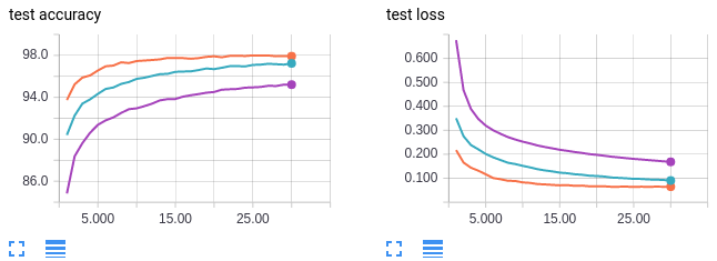
• Orange curves: batch size 64
• Blue curves: batch size 256
• Regal curves: batch size 1024

Finding: higher batch sizes leads to lower asymptotic exam accuracy.

The ten-axis shows the number of epochs of training. The y-axis is labelled for each plot. MNIST is plain an easy dataset to train on; we can attain 100% train and 98% test accuracy with just our base of operations MLP model at batch size 64. Further, we run into a clear trend between batch size and the asymptotic test (and train!) accuracy. We brand our first conclusion: higher batch sizes leads to lower asymptotic test accurateness. This patterns seems to exist at its extreme for the MNIST dataset; I tried batch size equals 2 and accomplished even better test accurateness of 99% (versus 98% for batch size 64)! As a forewarning, do not look very low batch sizes such as 2 to work well in more complex datasets.

Effect of Learning Rate

Finding: we can recover the lost test accuracy from a larger batch size past increasing the learning rate.

Some works in the optimization literature have shown that increasing the learning rate can compensate for larger batch sizes. With this in heed, we ramp up the learning rate for our model to see if we can recover the asymptotic test accuracy we lost by increasing the batch size.

Training loss and accurateness when the model is trained using dissimilar learning rates.

Testing loss and accuracy when the model is trained using different learning rates.

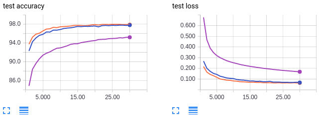
• Orange curves: batch size 64, learning charge per unit 0.01 (reference)
• Purple curves: batch size 1024, learning rate 0.01 (reference)
• Blue: batch size 1024, learning rate 0.1

The orangish and imperial curves are for reference and are copied from the previous set of figures. Like the imperial bend, the blue curve trains with a big batch size of 1024. Even so, the blue cure has a ten fold increased learning charge per unit. Interestingly we can recover the lost test accuracy from a larger batch size by increasing the learning charge per unit. Using a batch size of 64 (orangish) achieves a exam accuracy of 98% while using a batch size of 1024 merely achieves virtually 96%. But by increasing the learning charge per unit, using a batch size of 1024 also achieves examination accuracy of 98%. Just as with our previous conclusion, take this conclusion with a grain of salt. It is known that simply increasing the learning charge per unit does not fully compensate for big batch sizes in more circuitous datasets than MNIST.

Can you recover skillful asymptotic beliefs by lowering the batch size?

Finding: starting with a large batch size doesn't "get the model stuck" in some neighbourhood of bad local optimums. The model tin switch to a lower batch size or higher learning charge per unit anytime to reach better test accuracy.

The side by side interesting question to ask is whether training with large batch sizes "starts you lot out on a bad path from which you can't recover". That is, if we get-go training with batch size 1024, then switch to batch size 64, can we all the same attain the college asymptotic test accurateness of 98%? I investigated three cases: train using a small batch size for a single epoch so switch to a large batch size, railroad train using a small batch size for many epochs then switch to a larger batch size, and train using a big batch size then switch to a higher learning charge per unit with the same batch size.

Training loss and accuracy for different "recovery" scenarios.

Testing loss and accuracy for unlike "recovery" scenarios.

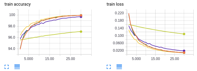
• Orange curves: railroad train on batch size 64 for 30 epochs (reference)
• Neon yellow: railroad train on batch size 1024 for threescore epochs (reference)
• Greenish curves: railroad train on batch size 1024 for i epoch then switching to batch size 64 for 30 epochs (31 epochs total)
• Dark yellow curves: train on batch size 1024 for 30 epochs then switching to batch size 64 for 30 epochs (60 epochs total)
• Royal curves: grooming on batch size 1024 and increasing the learning rate 10 folds at epoch 31 (60 epochs total)

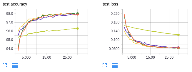
As before, the orange curves are for a small batch size. The neon yellow curves serve every bit a control to make sure we aren't doing improve on the test accurateness because nosotros're simply preparation more. If you pay careful attention to the 10-centrality, the epochs are enumerated from 0 to 30. This is because only the final 30 epochs of preparation are shown. For experiments with greater than 30 epochs of training in total, the commencement x − 30 epochs take been omitted.

Information technology's hard to come across the other 3 lines because they're overlapping but it turns out it doesn't matter because all 3 cases we recover the 98% asymptotic examination accurateness! In conclusion, starting with a large batch size doesn't "get the model stuck" in some neighbourhood of bad local optimums. The model tin can switch to a lower batch size or higher learning rate someday to achieve better test accurateness.

Hypothesis: gradient competition

Hypothesis: training samples in the same batch interfere (compete)
with each others' gradients.

How exercise we explain why training with larger batch sizes leads to lower test accurateness? I hypothesis might be that the training samples in the same batch interfere (compete) with each others' gradient. 1 sample wants to move the weights of the model in one management while another sample wants to move the weights the opposite direction Therefore, their gradients tend to cancel and you lot get a small overall gradients. Perchance if the samples are separate into two batches, and then competition is reduced as the model tin find weights that will fit both samples well if done in sequence. In other words, sequential optimization of samples is easier than simultaneous optimization in circuitous, high dimensional parameter spaces.

The hypothesis is represented pictorially below. The purple arrow shows a unmarried gradient descent pace using a batch size of 2. The bluish and blood-red arrows show ii successive gradient descent steps using a batch size of 1. The black arrow is the vector sum of the blue and red arrows and represents the overall progress the model makes in two steps of batch size ane. Both experiments start at the same weights in weight-space. While not explicitly shown in the prototype, the hypothesis is that the purple line is much shorter than the black line due to gradient competition. In other words, the gradient from a unmarried big batch size step is smaller than the sum of gradients from many small batch size steps.

Visualization of our gradient competition hypothesis.

The experiment involves replicating the picture shown higher up. We railroad train the model to a certain state. And then the control group (majestic arrow) is computed by finding the single-step gradient with batch size 1024. The experimental group (black arrow) is computed by making multiple gradient steps and finding the vector sum of those gradients using a smaller batch size. The production of the number of steps and batch size is fixed constant at 1024. This represents different models seeing a fixed number of samples. For case, for a batch size of 64 nosotros exercise 1024/64=16 steps, summing the 16 gradients to find the overall training gradient. For batch size 1024, nosotros do 1024/1024 = 1 step. Note that for the smaller batch sizes, different samples are fatigued for each batch. The idea is to compare the gradients of the model for different batch sizes after the models have seen the aforementioned number of samples. As a final caveat, for simplicity we but measure the gradient for the last layer of our MLP model which has 1024 ⋅ x = 10240 weights.

Nosotros investigated the following batch sizes: 1, ii, iii ,iv ,five, 6, 7, 8, sixteen, 32, 64, 128, 256, 512, 1024.

1 trial meant:

1. Loading/resetting the model weights to a fixed trained point (I used the model weights after training for two/30 epochs at 1024 batch size).
2. Randomly sampling 1024 data samples from the training set.
3. Step the model through all 1024 data samples one time, with different batch sizes.

For each batch size, I repeated the experiment 1000 times. I didn't have more data because storing the gradient tensors is really very expensive (I kept the tensors of each trial to compute college society statistics subsequently). The total size of the gradients tensor file was 600MB.

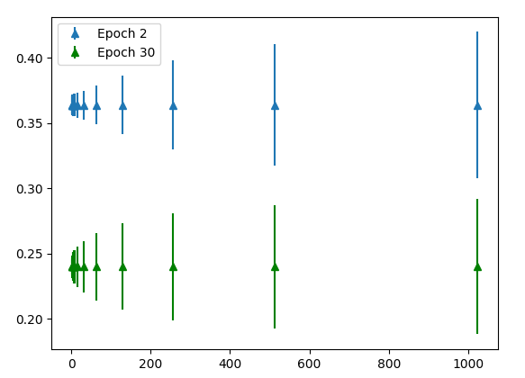
For each of the 1000 trials, I compute the Euclidean norm of the summed gradient tensor (black pointer in our movie). I then compute the mean and standard departure of these norms beyond the 1000 trials. This is washed for each batch size.

I wanted to investigate two dissimilar weight regimes: early on on during training when the weights have non converged and a lot of learning is occurring and afterward on during training when the weights have almost converged and minimal learning is occurring. For the early on regime, I trained the MLP model for 2 epochs with batch size 1024 and for the tardily regime, I trained the model for 30 epochs.

Boilerplate euclidean norm of slope tensors for dissimilar batch sizes at ii regimes: early on on during training and after during training.

Finding: larger batch sizes brand larger gradient steps than smaller batch sizes for the aforementioned number of samples seen.

The x-axis shows batch size. The y-centrality shows the average Euclidean norm of gradient tensors across m trials. The error bars indicate the variance of the Euclidean norm across 1000 trials. The blue points is the experiment conducted in the early on regime where the model has been trained for 2 epochs. The green points is the belatedly regime where the model has been trained for 30 epochs. As expected, the gradient is larger early during preparation (bluish points are higher than green points). Reverse to our hypothesis, the mean gradient norm increases with batch size! Nosotros expected the gradients to be smaller for larger batch size due to contest amongst data samples. Instead what we find is that larger batch sizes make larger gradient steps than smaller batch sizes for the aforementioned number of samples seen. Note that the Euclidean norm tin can be interpreted as the Euclidean distance between the new fix of weights and starting set of weights. Therefore, training with large batch sizes tends to move farther abroad from the starting weights afterwards seeing a stock-still number of samples than grooming with smaller batch sizes. The relation betwixt batch size and gradient norm is √x. In other words, the relationship between batch size and the squared gradient norm is linear.

Furthermore, the variance is much lower for smaller batch sizes. However, what we might intendance most is the magnitude of the variance relative to the magnitude of the mean. Therefore, to make a more insightful comparison, I calibration the both the mean and standard deviation of each batch size to the hateful of batch size 1024. In other words,

where the bars represent normalized values and i denotes a certain batch size.

Nosotros're justified in scaling hateful and standard deviation of the gradient norm considering doing and then is equivalent to scaling the learning rate up for the experiment with smaller batch sizes. Essentially we want to know "for the same distance moved abroad from the initial weights, what is the variance in slope norms for different batch sizes"? Keep in mind we're measuring the variance in the slope norms and not variance in the gradients themselves, which is a much effectively metric.

Normalized average euclidean norm of gradient tensors.

Finding: For the same average Euclidean norm distance from the initial weights of the model, larger batch sizes have larger variance in the distance.

We see a very surprising result above. For the aforementioned boilerplate Euclidean norm distance from the initial weights of the model, larger batch sizes accept larger variance in the distance. That's a mouthful! In brusk, given two models trained with different batch sizes, on any detail gradient footstep if the learning rate is adapted such that both models move on average the same distance, the model with the larger batch size will vary more than in how far information technology moves. This is somewhat counter-intuitive since it is well known that smaller batch sizes are "noisy" and therefore you might await the variance of the slope norm to be larger. Notation that for each trial we are sampling 1024 different samples, rather than using the same 1024 samples beyond all trials. Also note that the variance between trials might be caused by ii things: the different samples that are drawn from the dataset across different trials and the random seed for each trial (which wasn't controlled only really should be). Moving forwards, I'thou going to guess the variance is caused by the commencement factor: unlike samples. This is an interesting result and two things remain to be done:

1. Narrate the functional human relationship between batch size and the standard deviation of the average gradient norm.
2. Explicate why the variance increases with batch size.

Here'south the same analysis but we view the distribution of the entire population of 1000 trials. Each trial for each batch size is scaled using μ_1024/μ_i as before. The vertical axis is the batch size from 2 to 1024. The horizontal axis is the gradient norm for a particular trial. Due to the normalization, the center (or more accurately the mean) of each histogram is the same. The purple plot is for the early on regime and the blueish plot is for the belatedly regime.

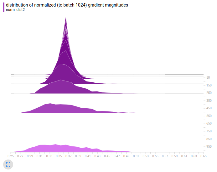
Finding: big batch size means the model makes very big slope updates and very minor gradient updates. The size of the update depends heavily on which particular samples are drawn from the dataset. On the other hand using small-scale batch size means the model makes updates that are all most the same size. The size of the update only weakly depends on which item samples are drawn from the dataset.

Nosotros see the aforementioned decision equally before: big batch size means the model makes very large slope updates and very small gradient updates. The size of the update depends heavily on which item samples are fatigued from the dataset. On the other mitt using small batch size means the model makes updates that are all about the aforementioned size. The size of the update but weakly depends on which item samples that are drawn from the dataset.

This conclusion is valid whether the model is in the early or late regime of preparation.

For reference, hither are the raw distributions of the gradient norms (same plots equally previously but without the μ_1024/μ_i normalization).

Finally permit's plot the raw gradient values without computing the Euclidean norm. What I've done hither is take each scalar slope in the gradient tensor and put them into a bin on the real number line. Nosotros combine the weights from the tensors of all 1000 trials by sharing bins between trials. As before, the vertical centrality represents the batch size. The horizontal axis represents the value of the gradient. Orangish is the early on government and low-cal bluish is the tardily regime.

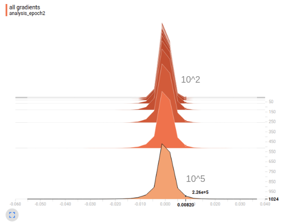
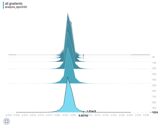
Finding: the distribution of gradients for larger batch sizes has a much heavier tail.

It'south hard to encounter, but at the particular value forth the horizontal axis I've highlighted nosotros meet something interesting. Larger batch sizes has many more large gradient values (about 10⁵ for batch size 1024) than smaller batch sizes (about x² for batch size 2). Note that the values have not been normalized past μ_1024/μ_i. In other words, the distribution of gradients for larger batch sizes has a much heavier tail. The number of large gradient values decreases monotonically with batch size. The heart of the gradient distribution is quite similar for different batch sizes. In conclusion, the gradient norm is on average larger for big batch sizes considering the gradient distribution is heavier tailed.

Next experiments: as I accept hinted, it might be interesting to wait at the functional human relationship between batch size and the variance of the average gradient norm and provide theoretical justification for the human relationship. Furthermore, nosotros might desire to analyze the direction of the gradients rather than only looking at the magnitude. We still tin't explain "increasing the learning rate recovers asymptotic examination accurateness."

Getting Far Enough

Hypothesis: larger batch sizes don't generalize as well considering the model cannot travel far plenty in a reasonable number of grooming epochs.

In the following experiment, I seek to answer why increasing the learning rate can compensate for larger batch sizes. We offset with the hypothesis that larger batch sizes don't generalize also because the model cannot travel far enough in a reasonable number of training epochs.

The experimental setup is simple. I start by preparation our model for 30 epochs. I then computed the L_2 distance betwixt the final weights and the initial weights. This experiment is designed under the assumption that maybe there are good optimas that are far away from the initial weights and certain grooming setups cannot achieve these optimas; they have to settle for worse optimas closer to the initial weights.

The vertical centrality represents dissimilar batch sizes (BS). The horizontal centrality represents different learning rates (LR). Each cell shows the altitude from the final weights to the initial weights (West), the altitude from the final biases to the initial biases (B) and the test accuracy (A).

Finding: amend solutions can be far away from the initial weights and if the loss is averaged over the batch then large batch sizes merely do not allow the model to travel far enough to reach the meliorate solutions for the aforementioned number of training epochs.

The best solutions seem to exist virtually ~vi distance abroad from the initial weights and using a batch size of 1024 we simply cannot reach that distance. This is because in about implementations the loss and hence the gradient is averaged over the batch. This means for a fixed number of training epochs, larger batch sizes take fewer steps. Even so, past increasing the learning charge per unit to 0.i, nosotros take bigger steps and tin can achieve the solutions that are farther away. In conclusion, meliorate solutions tin can be far away from the initial weights and if the loss is averaged over the batch then big batch sizes just do not allow the model to travel far enough to reach the improve solutions for the aforementioned number of grooming epochs. Interestingly, in the previous experiment we showed that larger batch sizes move further subsequently seeing the same number of samples.

To ostend our conclusion, I trained batch size 1024 using 0.01 learning rate for (1024/64) ⋅ 30 = 480 epochs. In this setup, the model takes the aforementioned number of full steps as it would if trained on batch size 64 for 30 epochs. Theoretically, this should let the model to travel to the far away solutions. Under this training setup, we find:

W: 6.63, B: 0.11, A: 98%

Indeed the model is able to find the far away solution and achieve the better test accuracy.

Finding: 1 can compensate for a larger batch size by increasing the learning rate or number of epochs so that the models tin can detect faraway solutions.

Here is a plot of the altitude from initial weights versus training epoch for batch size 64.

Distance from initial weights versus training epoch number for SGD.

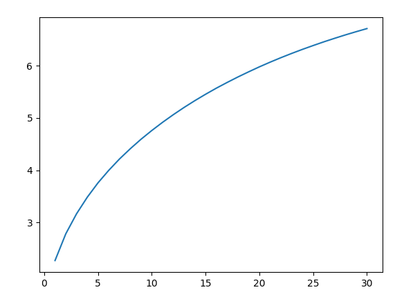
Finding: for a fixed number of steps, the model is limited in how far it can travel using SGD, independent of batch size.

The x-centrality represents the epoch number. The y-axis represents the distance from the initial weights. While the distance from initial weights increases monotonically over time, the rate of increase decreases. The plot for batch size 1024 is qualitatively the same and therefore now shown. Yet for the batch size 1024 case, the model tries to get far enough to detect a good solution but doesn't quite brand it. All of these experiments suggest that for a fixed number of steps, the model is limited in how far it can travel using SGD, independent of batch size.

Closing remarks: so far we've found that the reason smaller batch sizes railroad train more efficiently for the aforementioned number of epoch is because information technology takes more than steps. For a given number of steps, it seems like there'south an upperbound on how far the model can travel away from its original weights. Therefore, smaller batch sizes ways the model can notice the faraway, better optima whereas large batch size means the model cannot. However, from my own feel working with more complex datasets this can't be the whole story. I suspect that at that place are cases where the model travels only as far with a big batch size as a small-scale batch size but still does worse than smaller batch size. Furthermore, we recall the railroad train and test accuracy curves shown at the beginning of this study, they were both monotonically increasing. This is not representative of more than complex datasets where the training accuracy usually increases monotonically while the test accuracy starts decreasing from overfitting. This could be an important difference for why the conclusions of this study exercise non generalize to more complex datasets.

ADAM vs SGD

ADAM is i of the most popular, if not the almost popular algorithm for researchers to paradigm their algorithms with. Its claim to fame is insensitivity to weight initialization and initial learning charge per unit option. Therefore, information technology's natural to extend our previous experiment to compare the preparation behavior of ADAM and SGD.

Finding: ADAM finds solutions with much larger weights, which might explain why it has lower exam accuracy and is non generalizing every bit well.

Recall that for SGD with batch size 64 the weight distance, bias altitude, and test accuracy were 6.71, 0.11, and 98% respectively. Trained using ADAM with batch size 64, the weight distance, bias distance, and test accuracy are 254.iii, eighteen.three and 95% respectively. Notation both models were trained using an initial learning charge per unit of 0.01. ADAM finds solutions with much larger weights, which might explain why it has lower test accurateness and is non generalizing as well. This is why weight disuse is recommended with ADAM.

Here is the distance from initial weights for ADAM.

Distance from initial weights versus grooming epoch number for ADAM.

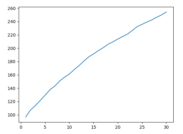
This plot is almost linear whereas for SGD the plot was definitely sublinear. In other words, ADAM is less constrained to explore the solution space and therefore tin can find very faraway solutions.

For perspective allow's find the distance of the final weights to the origin.

SGD

• batch size 64, Due west: 44.9, B: 0.11, A: 98%
• batch size 1024: W: 44.1, B: 0.07, A: 95%
• batch size 1024 and 0.1 lr: Westward: 44.vii, B: 0.10, A: 98%
• batch size 1024 and 480 epochs: W: 44.9, B: 0.xi, A: 98%

ADAM

• batch size 64: W: 258, B: xviii.3, A: 95%

Finding: for SGD the weights are initialized to approximately the magnitude y'all want them to be and well-nigh of the learning is shuffling the weights along the hyper-sphere of the initial radius. As for ADAM, the model completely ignores the initialization.

Nosotros deduce that for SGD the weights are initialized to approximately the magnitude you desire them to be (nigh 44) and most of the learning is shuffling the weights along the hyper-sphere of the initial radius (about 44). As for ADAM, the model completely ignores the initialization. Assuming the weights are also initialized with magnitude near 44, the weights travel to a final altitude of 258.

Finally permit's plot the cosine similarity between the final and initial weights. We have 3 numbers, ane for each of the 3 FC layers in our model.

SGD

• batch size 64, COS: [0.988 0.993 0.928]
• batch size 1024, COS: [0.998 0.998 0.978]
• batch size 1024 and 0.1 lr, COS: [ 0.991 0.994 0.936]
• batch size 1024 and 480 epochs, COS: [ 0.989 0.993 0.930]

ADAM

• batch size 64, COS: [ 0.124 0.359 0.153]

Again, we encounter that SGD leaves the initial weights almost untouched whereas ADAM completely ignores initialization. The second FC layer'south weights are appears to be the least changed (maybe considering the input and output layer learns to use the initialization of the second layer which shows the importance of a nonzero weight intialization: the model can merely utilize the randomness of some layers instead of needing to learn that layer).

In summary we fabricated the post-obit findings in our experiments:

• college batch sizes leads to lower asymptotic exam accuracy
• we can recover the lost test accuracy from a larger batch size by increasing the learning rate
• starting with a large batch size doesn't "get the model stuck" in some neighbourhood of bad local optimums. The model tin can switch to a lower batch size or higher learning charge per unit someday to achieve improve examination accuracy
• larger batch sizes brand larger gradient steps than smaller batch sizes for the same number of samples seen
• for the same average Euclidean norm altitude from the initial weights of the model, larger batch sizes have larger variance in the distance.
• large batch size means the model makes very large gradient updates and very small slope updates. The size of the update depends heavily on which particular samples are drawn from the dataset. On the other hand using pocket-size batch size means the model makes updates that are all about the same size. The size of the update only weakly depends on which particular samples are drawn from the dataset
• the distribution of gradients for larger batch sizes has a much heavier tail
• improve solutions tin be far abroad from the initial weights and if the loss is averaged over the batch and then large batch sizes but practise non allow the model to travel far enough to attain the better solutions for the aforementioned number of training epochs
• one tin recoup for a larger batch size by increasing the learning rate or number of epochs so that the models can discover faraway solutions
• for a fixed number of steps, the model is limited in how far it can travel using SGD, independent of batch size
• ADAM finds solutions with much larger weights, which might explain why information technology has lower test accurateness and is non generalizing besides
• for SGD the weights are initialized to approximately the magnitude y'all desire them to be and most of the learning is shuffling the weights along the hyper-sphere of the initial radius. As for ADAM, the model completely ignores the initialization

Equally I mentioned at the start, training dynamics depends heavily on the dataset and model and so these conclusions are signposts rather than the last word in understanding the effects of batch size.

Source: https://medium.com/mini-distill/effect-of-batch-size-on-training-dynamics-21c14f7a716e

Posted by: bowdenheman1981.blogspot.com

Share this post